Gradient Descent Algorithm

Table of Contents

The gradient descent algorithm is an iterative derivative-based local optimisation search algorithm that aims to find the optimum vector value that minimises the objective or cost function. For those not familiar with optimisation theory, the gradient descent algorithm aims to find the coordinate location where a given function (i.e. the objective function) is at its lowest value. Such a point is called the “optimum” or “minimum” point.

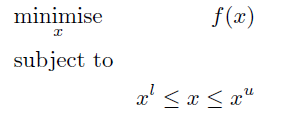
Gradient descent - iterative search formula

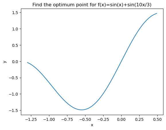
A solution technique must thus be devised to find the value of x that will correspond to the smallest value of f. One such technique for differentiable functions is to use the gradient descent algorithm, that is, given an initial x_0 value, a search direction must be devised to iteratively get closer to the optimum point. Using gradient information can help reach such a point, as the gradient provides information on the direction of the steepest descent or slope:

Thus this iterative update of the initial guess continues repeatedly until a stopping criterion is reached. Typically, the algorithm is stopped when the derivative of the function nears zero and does not significantly change over time.

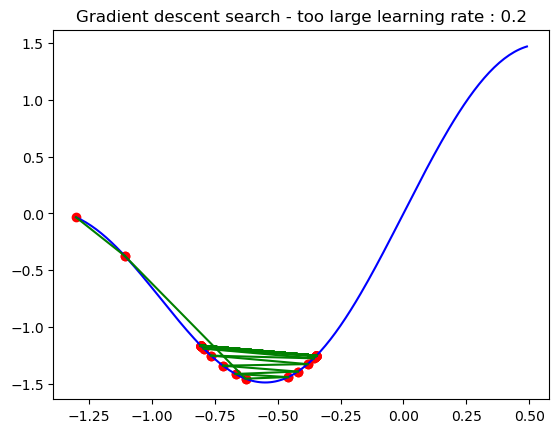
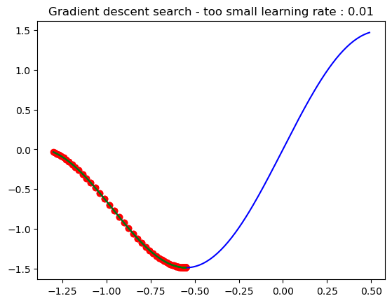
Although the algorithm is simple, the choice of the learning rate is critical to the success of the search. A too-small learning rate would slow down the search and thus waste time while a too-large learning rate would lead to jumping far away from the optimum point and eventually missing it.

Python Implementation

import numpy as np
import matplotlib.pyplot as plt

#objective function
def obj_func(x):
    y = np.sin(x) + np.sin((10.0 / 3.0) * x)
    return y
#compute the derivative function
def derivate_func(x):
    dx = np.cos(x) + (10/3)*np.cos((10.0/3.0)*x)
    return dx
#search bounds
x_l = -1.3
x_u = 0.5
#function data
x_i = np.arange(x_l,x_u,step=0.01)
y_i = obj_func(x_i)
plt.figure()
plt.xlabel('x')
plt.ylabel('y')
plt.plot(x_i,y_i)
plt.title('Find the optimum point for f(x)=sin(x)+sin(10x/3)')
plt.show()

#Gradient descent algorithm
N_search_iters = 100 #number of search steps
x_n = x_l #initial value
gamma = 0.05 #learning rate

plt.figure()
plt.plot(x_i,y_i,color="blue")
for i in range(N_search_iters):
    x_np = x_n - gamma*derivate_func(x_n) #gradient descent search formula
    x_0 = x_n#gathering data points
    x_1 = x_np #gathering data points
    #update x_n
    x_n = x_np
    #plotting search points
    y_0 = obj_func(x_0)
    y_1 = obj_func(x_1)
    plt.scatter(x_0,y_0,color="red")
    plt.scatter(x_1,y_1,color="red")
    plt.plot([x_0,x_1],[y_0,y_1],color="green")
    
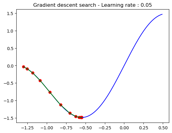
plt.title('Gradient descent search - Learning rate : 0.05')
plt.show()
x_optimum = x_n
y_opt = obj_func(x_optimum)
print("x-optimum:%.3f f-optimum:%.3f"%(x_optimum,y_opt))

Using a balanced learning rate (i.e. 0.05) and the gradient iterative search the optimum point is obtained x=-0.549, which is the point where the function reaches its smallest value f=-1.488.

Gradient descent algorithm in Machine learning

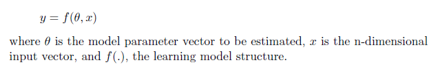
The gradient descent algorithm is typically used in machine learning to estimate model parameters. Given, a generic learning model of the type

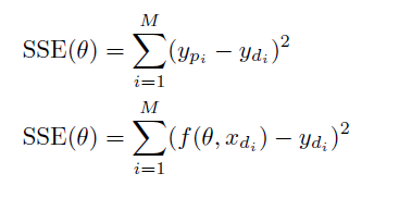
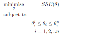
A cost function that aims to minimise the sum of square error between the model prediction (y_p) and the actual observation data (y_d) is often built to estimate the most appropriate model parameters.

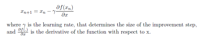
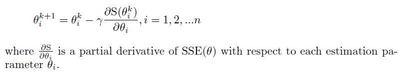
The optimisation problem below is thus formulated and commonly solved using the gradient descent algorithm.

leading to a more generic gradient search update formula that takes into account multiple parameter estimates:

This algorithm is often built into several machine-learning packages and automatically used during the training process.

Limitations of the Gradient descent algorithm

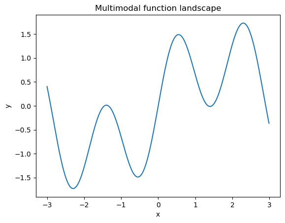
One pertinent limitation of the gradient descent algorithm is that it can guarantee the obtention of the true optimum when only the function has one convex lobe. For multimodal functions, with multiple potential optima, the gradient descent algorithm can only obtain the (local) optimum near the initial guess. Nevertheless, this is not a major challenge in machine learning which settles with obtaining a good enough relative minimum as aiming to find the global optimum is unpractical and generally very resource intensive.

Conclusion

The gradient descent algorithm is a simple iterative derivative-based local optimisation algorithm commonly used in machine learning for model training (i.e. parameter estimation). The algorithm makes use of gradient information of the objective function to lead the search towards the optimum point of minimisation. The choice of the learning rate is crucial to the speed and success of the search algorithm, often requiring that the model input vectors be normalised in order to set a generic balanced learning rate. More advanced parameter search algorithms such as particle swarm optimisation and other metaheuristics are sometimes used when it is crucial to find the global optimum to yield some improvement in the model pattern recognition performance.

Author: Yves Matanga, PhD

Be the first to receive notification, when new content is available!

Post Views: 1,280