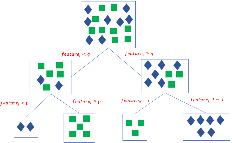
Decision Trees are universal approximators that learn (nonlinear) patterns in the data based on a rule-based inference process that forms by recursive splitting homegenous data subgroups representing the same target class or sharing similar target values. Given a dataset of n features and m records, the decision tree iteratively selects the most informative feature and splits the datasets repeatedly into near-homogenous labelled subcategories until a stopping criterion is met.
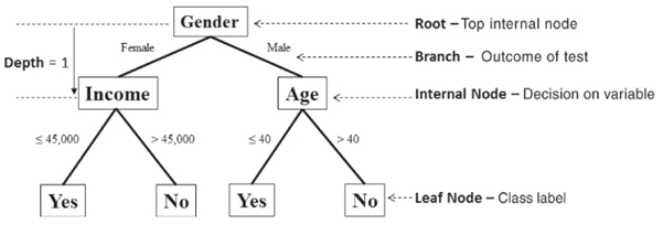
The top node is referred to as the root node and is the starting decision node. (i.e., Gender is Male or Female?). A branch is a subset of the dataset obtained as an outcome of a test. Internal nodes are decision nodes based on which subsequent branches are obtained. The depth of a node is the minimum number of decisions it takes to reach it from the root node. The leaf nodes are the end of the last branches on the tree which determine the output (class label or regression value).
Example of a Decision Tree for Classification [EMC, Data Science and Big Data Analytics]
Building a decision tree
Given a dataset of n features and m records, a rule-based graph is formed iteratively by recursive partitioning until the datasets is split in homogenous data groups representing the same target class in a classification problem or sharing close target values in a regression problem . From the root node (i.e. with all the m records), the most informative attribute is identified using some feature important score. The Gini index is the most commonly used feature importance score among others (entropy, information gain):
which measures the probability of a dataset to purely separated in its distinct classes upon a split on the given feature. It thus gauges the importance of a feature f in distinguishing classes in a given dataset. The lower the Gini index, the more likely the dataset classes are separable by the selected feature split, the higher the Gini index the less likely the dataset classes are separable by the selected feature split. Thus, in any given data subset, the feature with the lowest gini index is selected. In a practical implementation of a typical binary decision tree, the Gini index upon a given feature split, will be computed as a weighted sum of the gini indexes in each subset:
In the same vein, for a regression problem, the quality of the split is measured using some measure within subset target values closeness such as the mean square error or variance.
Given an appropriate feature importance selection criterion, the decision tree is thus built as follows by recursive partitioning.
Step 1: Given M attributes in a dataset N records and a target variable y
Step 2: Rank features as per the chosen feature importance score
Step 3: Split the dataset by the feature with the best importance score
Step 4: Repeat Step 2 to each new subset until a stopping criterion is met
Recursive partitioning stops when either the minimum number of samples per subset is reached, when a data subset is homogenous or near homogenous by some degree or when the node has a maximum preset depth.
Pruning a decision tree
The recursive nature of building decision trees renders the algorithm prone to overfitting. A decision tree can reach 100% fitting accuracy on the training set given that it can further split the data until a single data (i.e. guaranteed homogeneity) remains. However, this comes with the risk that the algorithm may lose its generalisation capability on unseen data. A pruning phase may post-process the decision tree, undermine some rules and allow some level of heterogeneity in the data subgroups to secure generalisation on unseen data.
Python Implementation - Classification problem
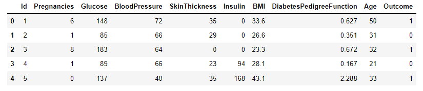
A sample dataset for diabetes classification [1] will be used to test the performance of decision trees as a binary classifier. Data were extracted from 2768 patient records with mixed data of healthy and non-healthy patients inclusive of nine attributes:
Id: Unique identifier for each data entry.
Pregnancies: Number of times pregnant.
Glucose: Plasma glucose concentration over 2 hours in an oral glucose tolerance test.
BloodPressure: Diastolic blood pressure (mm Hg).
SkinThickness: Triceps skinfold thickness (mm).
Insulin: 2-Hour serum insulin (mu U/ml).
BMI: Body mass index (weight in kg / height in m^2).
DiabetesPedigreeFunction: Diabetes pedigree function, a genetic score of diabetes.
Age: Age in years.
Outcome: Binary classification indicating the presence (1) or absence (0) of diabetes.
#-- Load the Dataset
import pandas as pd
import warnings
warnings.filterwarnings('ignore') #ignore warnings
df = pd.read_csv('https://raw.githubusercontent.com/mlinsights/freemium/main/datasets/classification/diabetes/Healthcare-Diabetes.csv')
df.head()
#-- Summarise the Dataset
df.info()
#-- Extract Features and the target variable
X = df.iloc[:,1:9]
y = df[['Outcome']]
#-- Split the Dataset in Training and Test Set
from sklearn.model_selection import train_test_split
X_train, X_test, y_train, y_test = train_test_split(X,y,test_size=0.2,random_state=1234)#fix the random seed (to reproduce the results)
#-- Training the model
from sklearn.tree import DecisionTreeClassifier
import matplotlib.pyplot as plt
from sklearn import tree
dt_classifier = DecisionTreeClassifier(criterion="gini",max_depth=2,min_samples_leaf=1)#Setting the decision tree - settings
dt_classifier.fit(X_train,y_train)#train the classifier
tree.plot_tree(dt_classifier)
plt.show()
# -- Benchmark the model performance
from sklearn.metrics import confusion_matrix
from sklearn.metrics import classification_report
import seaborn as sns
import numpy as np
y_pred_train = dt_classifier.predict(X_train)
y_pred_test = dt_classifier.predict(X_test)
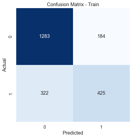
# Create confusion matrix for the training set
cm_train = confusion_matrix(y_train, y_pred_train)
# Create heatmap - Test set
plt.figure(figsize=(8, 6))
sns.set(font_scale=1.2)
sns.heatmap(cm_train, annot=True, fmt="d", cmap="Blues", cbar=False, square=True)
plt.xlabel('Predicted')
plt.ylabel('Actual')
plt.title('Confusion Matrix - Train')
plt.show()
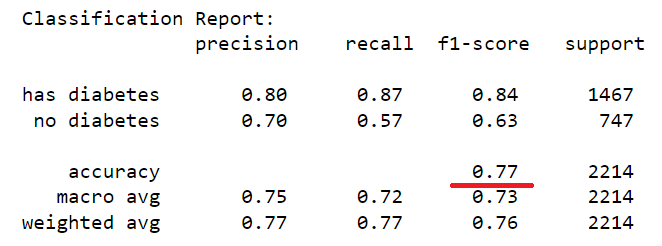
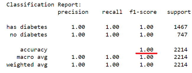
train_report = classification_report(y_train, y_pred_train, target_names=['has diabetes','no diabetes'])
print("Classification Report:\n", train_report)
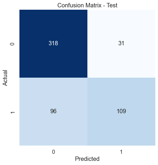
# Create confusion matrix test set
cm_test = confusion_matrix(y_test, y_pred_test)
# Create heatmap - Test set
plt.figure(figsize=(8, 6))
sns.set(font_scale=1.2)
sns.heatmap(cm_test, annot=True, fmt="d", cmap="Blues", cbar=False, square=True)
plt.xlabel('Predicted')
plt.ylabel('Actual')
plt.title('Confusion Matrix - Test')
plt.show()
#tn, fp, fn, tp = cm_test
class_acc = (cm_test[0][0]+cm_test[1][1])/(cm_test[0][0]+cm_test[0][1]+cm_test[1][0]+cm_test[1][1])
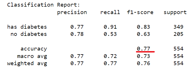
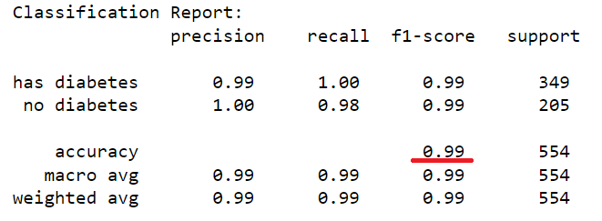
test_report = classification_report(y_test, y_pred_test, target_names=['has diabetes','no diabetes'])
print("Classification Report:\n", test_report)
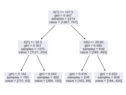
The dataset of records is split into training and test (80/20) to test the predictive performance of the decision tree in distinguishing between the presence or absence of diabetes. The model will thus be trained on the training set alone but benchmarked on the training and test set. The test performance being the most important has it is an indicator of the model predictive power on unseen data. Having fixed the maximum tree depth to 2, the decision tree rules can be visualised clearly. For performance sake, the maximum depth can be set to None to alow maximum insight discovery. With the current settings, the model classification performances are recorded and presented in the figure below.
After lifting the restriction of the search of the decision tree (i.e. max-depth = None), a fully blown decision tree classifier is obtained with excellent performance illustrating the outstanding predictive capabilities of the algorithm.
dt_classifier = DecisionTreeClassifier(criterion="gini",max_depth=None,min_samples_leaf=1)#Setting the decision tree - settings
dt_classifier.fit(X_train,y_train)#train the classifier
Python Implementation - Regression problem
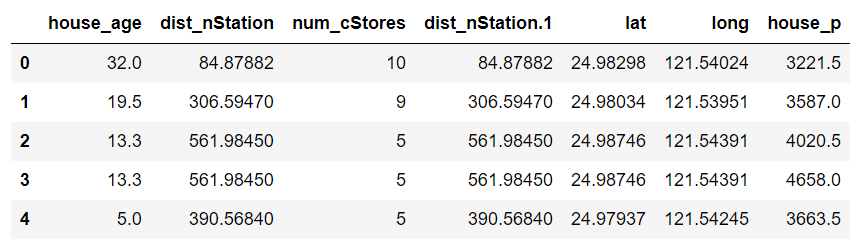
To illustrate the performance of the decision for regression, a dataset of 414 records of house pricing data in a given region is used. The dataset consists of six attributes: the house’s distance to the nearest train station, the number of convenience stores surrounding the house as well as the latitude and longitude location of the house. The target variable is the house sold price per square meter. A regression model must thus be built to learn the inherent house pricing strategy used in the area.
#--load the datasets
import pandas as pd
import warnings
warnings.filterwarnings('ignore') #ignore warnings
df = pd.read_csv('https://raw.githubusercontent.com/mlinsights/freemium/main/datasets/regression-analysis/real-estate-house-pricing/real_estate_data.csv')
df = df.iloc[:,1:] #retrieve house pricing data
df.head()
#get the datasets description
df.info()
#--extract features and the target variable
X = df.iloc[:,0:6]#get features
y = df.iloc[:,[6]]#get target variable
X.head()
#--Split the the training set from the test set
from sklearn.model_selection import train_test_split
X_train, X_test, y_train, y_test = train_test_split(X,y,test_size=0.2,random_state=1234)#fix the random seed (to reproduce the results)
#--Build the Decision Tree Regression model
from sklearn.tree import DecisionTreeRegressor
import matplotlib.pyplot as plt
from sklearn import tree
dt_regressor = DecisionTreeRegressor(criterion="squared_error",max_depth=None,min_samples_leaf=1)#Setting the decision tree - settings
dt_regressor.fit(X_train,y_train)#train the classifier
tree.plot_tree(dt_regressor) #display the model rules
plt.show()
#--Compute the Coefficient of determination and visualise the goodness of fit for both the training and test setfrom sklearn.metrics import r2_score
y_pred_train = dt_regressor.predict(X_train)#get model prediction on training set
y_pred_test = dt_regressor.predict(X_test)#get model prediction on test
r2_score_train = r2_score(y_train,y_pred_train)
r2_score_test = r2_score(y_test,y_pred_test)
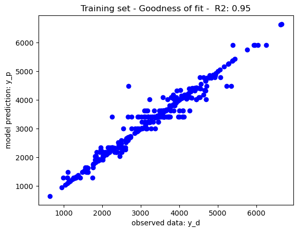
plt.figure()
plt.scatter(y_train, y_pred_train, color="b")
plt.xlabel('observed data: y_d')
plt.ylabel('model prediction: y_p')
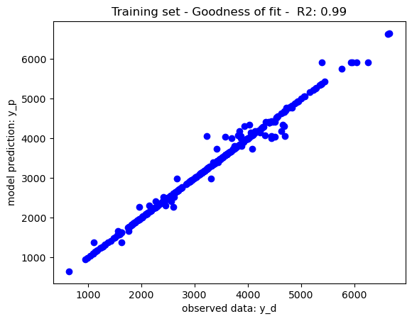
plt.title('Training set - Goodness of fit - R2: %.2f'%r2_score_train)
plt.show()
plt.figure()
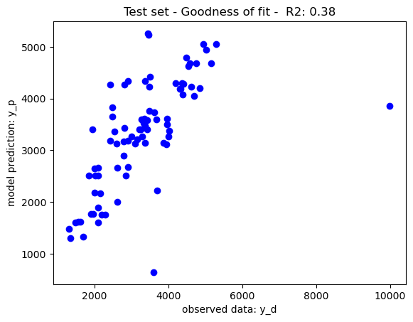
plt.scatter(y_test, y_pred_test, color="b")
plt.xlabel('observed data: y_d')
plt.ylabel('model prediction: y_p')
plt.title('Test set - Goodness of fit - R2: %.2f'%r2_score_train)
plt.show()
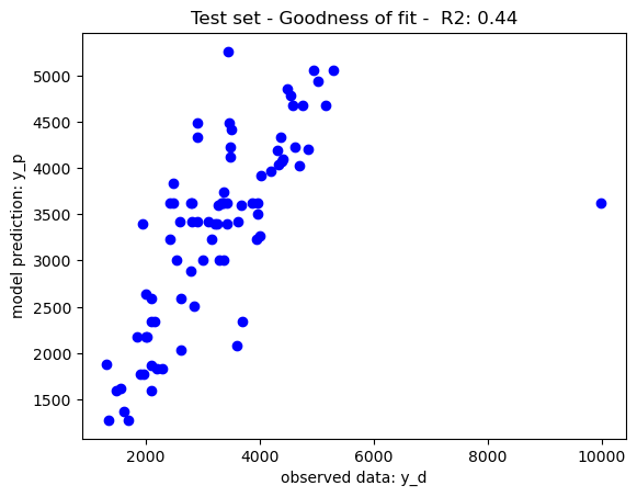
The mean square error has been to rank features, the decision trees have been trained with limits of node depth and a minimum leaf node size of 1, yielding the goodness of fit recorded in the below graphs. As per theory, the training set performance have tendencies to overfit yield a near perfect which may impact on its generalisation prowesses. The performance on the test set may be due to either overfitting or the complexity of the dataset. To further improve the model performance, a hyperparameter tuning may be use to tune the decision tree parameters to its best performing configuration (i.e. max depth, min leaf node size, etc.)
Illustratively, reducing the maximum depth of node split to 10 has balanced the tradeoff between training and generalisation further boosting the model performance on the test set. Feature selection may also be considered to further boost the model performance. Nevertheless, as per the No Free Lunch Theorem, other nonlinear models may also be considered given that different models perform differently on different datasets.
dt_regressor = DecisionTreeRegressor(criterion="squared_error",max_depth=10,min_samples_leaf=1)#Setting the decision tree - settings
dt_regressor.fit(X_train,y_train)#train the regression model
Conclusion
Decision Trees are powerful universal approximators that can be used for both regression and classification. The algorithm generates a rule-based tree of the inherent pattern in the datasets by recursively partitioning the dataset on the informative features per data subset until it separates the original data into homogenous or near-homogeneous groups. It is a nonparametric model that can identify very complex linearities in datasets. Nevertheless, extra care should be taken to control the model training process (i.e. node splitting) and avoid overfitting that may impede on its accuracy on unseen data. Hyperparameter tuning or posterior tree pruning phase may be used to achieve such a fit.