Linear Regression

Linear regression is the most basic regression algorithm that assumes the existence of a linear relationship between the independent variable and the dependent variables. 

Albeit its basic relationship model, it is a powerful technique robust to noise that can estimate a skeletal relationship in labelled data.
Given the fictional dataset below of a survey data of different competitors of milk price settings, a regression model could be built to estimate the inherent relationship.

A linear regression model can be applied to the given datasets and estimate the inherent relationship which will come down to estimate the linear model parameters as show in the equation below.

This leads to the derivation of the estimated model illustrated in the Figure below: p(g) = 0.111g + 19.861, which accurately describes the relationship in the dataset.

Model estimation Formulation

Given a set of M observations of labelled data (xdi , ydi ) with n dependent variables, the model parameters below can be estimated using the least square estimation method.

linear regression equation

which requires finding the model parameters that will minimise the sum of square error (SSE) between the target output observation values and the model prediction.

sum of square error

Utilizing the gradient descent algorithm is a common approach to minimize this cost function (SSE(θ)) and estimate the model parameters. For datasets of manageable size, a direct estimation approach employing matrix manipulation is also viable. Interested readers can look at Appendix A of the work at the following link.

Python implementation
import pandas as pd
import matplotlib.pyplot as plt
import warnings
warnings.filterwarnings('ignore') #ignore warnings

df = pd.read_csv('https://raw.githubusercontent.com/mlinsights/freemium/main/datasets/regression-analysis/milk_price_market_survey.csv')
df.head()

plt.figure() #plotting the data
plt.scatter(df['gram'],df['price'])
plt.xlabel('gram (g)')
plt.ylabel('unit price')
plt.title('Milk Pricing Survey Data')

from sklearn.linear_model import LinearRegression
import numpy as np

lm = LinearRegression()
X = df[['gram']]
y = df[['price']]

lm.fit(X,y) #fit model
y_predict = lm.predict(X)#get model prediction of observation
price_model = "p(g) = %.3fg + %.3f"%(lm.coef_[0],lm.intercept_)
print(price_model)

x_min = X.min()[0] #find variable lower bound
x_max = X.max()[0] #find variable upper bound
r_x = x_max-x_min
x_n = np.arange(x_min,x_max,step=r_x/100) 
y_n = lm.predict(x_n.reshape(-1,1))

plt.figure()
plt.scatter(df['gram'],df['price'])
plt.plot(x_n,y_n,color="red")
plt.xlabel('gram (g)')
plt.ylabel('unit price')
plt.title('Milk Pricing Survey Data - Regression model: %s'%(price_model))
plt.show()

 
Goodness of fit and R2 score
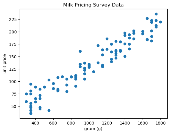
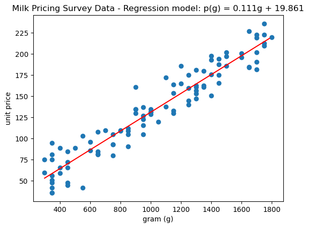
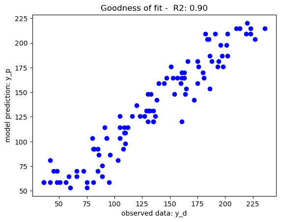
To evaluate the goodness of fit for a regression model, a scatter plot displaying observed data and model predictions is often created, accompanied by the coefficient of determination score R2. A well-fitted model will yield a stronger correlation between observed data and the model prediction.
from sklearn.metrics import r2_score

r2_score_m = r2_score(y_predict,y)

plt.figure()
plt.scatter(y, y_predict, color="b")
plt.xlabel('observed data: y_d')
plt.ylabel('model prediction: y_p')
plt.title('Goodness of fit -  R2: %.2f'%r2_score_m)
plt.show() 
Conclusion

Linear regression is a simple regression model that assumes a linear relationship between dependent variables and the target output using, most typically the least square estimation approach to determine the model parameters. It is robust in estimating the skeletal relational in simple and complex datasets.  Nonlinear regression models can be used to estimate more intricate relationships when the data inherent connections are nonlinear.

Author: Yves Matanga, PhD

Be the first to receive notification, when new content is available!

Leave a Reply

Your email address will not be published. Required fields are marked *