Logistic Regression is a classification method that models the probability of binary outcomes using the logistic function on a linear combination of the input features. Binary classification can be viewed as a machine learning attempt to estimate the conditional probability of obtain a class A given a feature vector:
\[P(Y=1|X=x) = f(\theta,x) \]
In logistic regression, this probability distribution is estimated using the sigmoid function on a linear combination of features.
\[P(Y=1|X=x) = \frac{1}{1+e^{-z}}, z = \theta_0 + \sum_{i=1}^{n}\theta_ix_i\]
To estimate the model parameters, the maximum likelihood estimation method is used. This method aims to find the model parameters that will maximise the joint probability of obtaining all data points x_i in their corresponding class y_i from the given dataset.
Using the gradient descent algorithm or a similar local optimisation method, the derived cost function can be maximised leading to the obtention of the model parameters.
Python Implementation
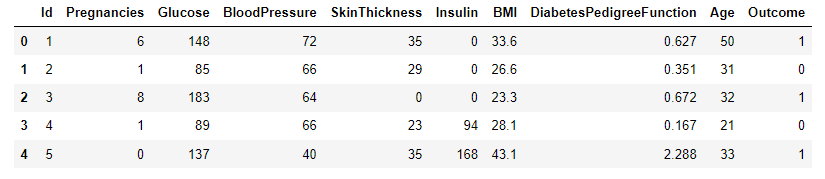
A sample dataset for diabetes classification [1] will be used to test the performance of kNN as a binary classifier. Data were extracted from 2768 patient records with mixed data of healthy and non-healthy patients inclusive of nine attributes:
Id: Unique identifier for each data entry.
Pregnancies: Number of times pregnant.
Glucose: Plasma glucose concentration over 2 hours in an oral glucose tolerance test.
BloodPressure: Diastolic blood pressure (mm Hg).
SkinThickness: Triceps skinfold thickness (mm).
Insulin: 2-Hour serum insulin (mu U/ml).
BMI: Body mass index (weight in kg / height in m^2).
DiabetesPedigreeFunction: Diabetes pedigree function, a genetic score of diabetes.
Age: Age in years.
Outcome: Binary classification indicating the presence (1) or absence (0) of diabetes.
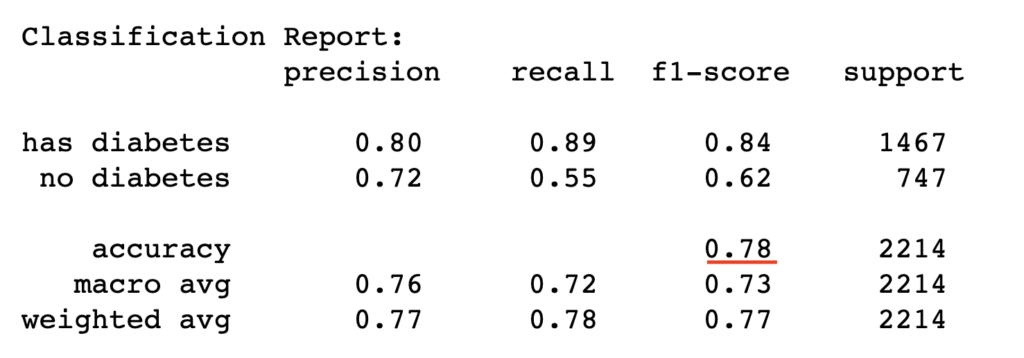
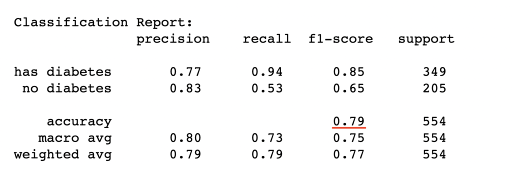
The dataset of records is split into training and test (80/20) to test the predictive performance of logistic regression in distinguishing between the presence or absence of diabetes. The model will thus be trained on the training set alone but benchmarked on the training and test set. The test performance is the most important as it indicates the model’s predictive power on unseen data.
import pandas as pd
import warnings
warnings.filterwarnings('ignore') #ignore warnings
df = pd.read_csv('https://raw.githubusercontent.com/mlinsights/freemium/main/datasets/classification/diabetes/Healthcare-Diabetes.csv')


X = df.iloc[:,1:9]
y = df[['Outcome']]

from sklearn.model_selection import train_test_split

X_train, X_test, y_train, y_test = train_test_split(X,y,test_size=0.2,random_state=1234)#fix the random seed (to reproduce the results)


from sklearn.linear_model import LogisticRegression

clf = LogisticRegression()
clf.fit(X_train,y_train)#train the classifier
#get model prediction on train set and test set
y_pred_train = clf.predict(X_train)
y_pred_test = clf.predict(X_test)


from sklearn.metrics import confusion_matrix
from sklearn.metrics import classification_report

import matplotlib.pyplot as plt
import seaborn as sns
import numpy as np

# Create confusion matrix for the training set
cm_train = confusion_matrix(y_train, y_pred_train)

# Create heatmap - Test set
plt.figure(figsize=(8, 6))
sns.set(font_scale=1.2)
sns.heatmap(cm_train, annot=True, fmt="d", cmap="Blues", cbar=False, square=True)
plt.xlabel('Predicted')
plt.ylabel('Actual')
plt.title('Confusion Matrix - Train')
plt.show()

train_report = classification_report(y_train, y_pred_train, target_names=['has diabetes','no diabetes'])
print("Classification Report:\n", train_report)


# Create confusion matrix test set
cm_test = confusion_matrix(y_test, y_pred_test)
# Create heatmap - Test set
plt.figure(figsize=(8, 6))
sns.set(font_scale=1.2)
sns.heatmap(cm_test, annot=True, fmt="d", cmap="Blues", cbar=False, square=True)
plt.xlabel('Predicted')
plt.ylabel('Actual')
plt.title('Confusion Matrix - Test')
plt.show()

#tn, fp, fn, tp = cm_test
class_acc = (cm_test[0][0]+cm_test[1][1])/(cm_test[0][0]+cm_test[0][1]+cm_test[1][0]+cm_test[1][1])
test_report = classification_report(y_test, y_pred_test, target_names=['has diabetes','no diabetes'])
print("Classification Report:\n", test_report)
Conclusion
Logistic regression is a powerful classification method that gives decent classification results based on the datasets under investigation. However, the model performance depends on whether the logistic function assumption of linearity in features holds, which may not hold for every use case. In such cases, the model may be improved using nonlinear logistic regression that rather assumes complex nonlinear relationship in the features.