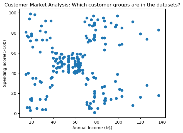
K-means clustering is a simple and popular clustering algorithm that groups data into k-groups of clusters whereby the value of k must be given apriori. It is used in several applications such as customer market analysis or object recognition whereby the inherent grouping in the data needs to be discovered based on some properties in the data. The figure shows a typical clustering problem of a store that would like to find the different groups of customers they have based their spending scores and annual incomes, a 2D clustering problem. In K-Means clustering the value of k needs to be set a priori (i.e k=3) and the algorithm would identify the most fitting data mapping in k-clusters.
Mathematical formulation
Given a set of N data vectors and a priori k value, the algorithm aims to determine a decent grouping of the data points in k clusters using a cost function that minimises the within-cluster sum of square error or variance (WCSS):
A fundamental heuristic algorithm to estimate the centroid locations (i.e mi) is through the use of Lyod’s algorithm. It is an iterative approach in which an initial guess of centroid vectors is set, followed by a clustering phase of data points around their closest centroids, leading to the mean estimation of new centroid locations. This process continues iteratively until the new estimated centroid locations do not significantly vary.
LLoyd's algorithm
Python implementation
import pandas as pd
import matplotlib.pyplot as plt
import warnings
warnings.filterwarnings('ignore') #ignore warnings
#load the dataset
df = pd.read_csv('https://raw.githubusercontent.com/mlinsights/freemium/main/datasets/clustering/OLART_customers.csv')
df.head()


#select data of interest
sub_df = df.iloc[:,[3,4]] #Annual Income against Spending Score
x_1 = sub_df['Annual Income (k$)']
x_2 = sub_df['Spending Score (1-100)']

#plotting the data of interest
plt.figure()
plt.scatter(x_1,x_2)
plt.xlabel('Annual Income (k$)')
plt.ylabel('Spending Score(1-100)')
plt.title('Annual Income (k$) vs Spending Score')
plt.show()

#Perform K-Means clustering
from sklearn.cluster import KMeans

k_choice = 3 #choice of k
km = KMeans(k_choice)
clusterIds = km.fit_predict(sub_df) #get data group labels

plt.figure()
plt.xlabel(sub_df.columns[0])
plt.xlabel(sub_df.columns[1])
plt.scatter(x_1,x_2,c=clusterIds)
plt.title('OLART - customer analysis: k = 3')
plt.show()
Estimating the optimal number of clusters - The Elbow method
Several methods have been proposed in the literature to estimate the optimal k. The elbow method is a graphical and first estimation method that every data analyst should know. It consists of computing the WCSS for a range of k and selecting the k-value where the sharpest bend occurs as the optimal k value. The rationale of this rationale is that the sharpest bend is the point of the most drastic improvement in within-in cluster variance beyond which any drop in WCSS is insignificant.
In the given dataset, the sharpest bend occur at k equals to 5, and thus k-Means will generate 5 cluster groups accordingly.
import numpy as np

wcss = []
for k in range(1,20): #set range k values to search from
    km = KMeans(k)
    km.fit(sub_df)
    wcss_iter = km.inertia_ #store the WCSS per the current k
    wcss.append(wcss_iter)

plt.figure()
plt.plot(np.arange(1,20),wcss)
plt.xticks(range(1,20))
plt.xlabel('k values')
plt.ylabel('WCSS(k)')
plt.title('Optimal k estimation - Elbow method')
plt.show()

k_optimal = 5  #sharpest bend at k=5
km = KMeans(k_optimal)
clusterIds = km.fit_predict(sub_df) #get data group labels

plt.figure()
plt.xlabel(sub_df.columns[0])
plt.xlabel(sub_df.columns[1])
plt.scatter(x_1,x_2,c=clusterIds)
plt.title('OLART - customer analysis: k = %d'%k_optimal)
plt.show()
Conclusion
K-Means clustering is a popular clustering algorithm generally effective for data that exhibits spherical cluster geometry. Given the sensitivity of the algorithm to initial centroid locations, the training process is often re-run several times to minimise potential bias into suboptimal locations. More robust techniques exist in the literature that uses metaheuristic search algorithms to improve its stability and more advanced non-graphical estimation k-estimation approaches are also used. Nevertheless, the use of the technique in its classic formulation remains popular and pertinent in data analytics applications.
Author: Yves Matanga, PhD
Be the first to receive notification, when new content is available!