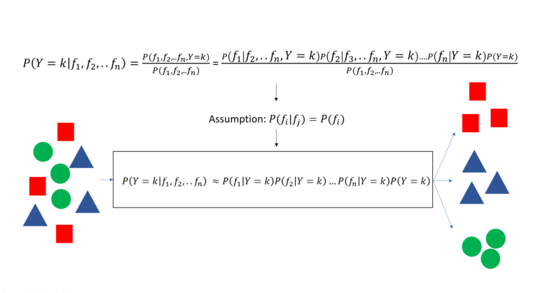
The Naive Bayes classifier is a classification method that takes the assumption of independence in features to relax the Bayes theorem and build a classification method.
\[P(B|A) = \frac{P(A \cap B) }{P(A)} = \frac{P(A|B)P(B)}{P(A)}\]
This relaxation drastically simplifies the computation of the conditional probability P(Y|X) which now only depends on the conditional probabilities P(x_i|Y=k) and the joint probability of features.
The second simplification of the Naive Bayes theorem is to disregard the joint probability of features P(x_1,x_2,..x_n) as this probability is a constant and equally comparable when assessing a given vector belongingness among each class k.
Thus the Naive Bayes classifier does not compute true probability but rather a probability-based score to assign a data point to the most probable class.
For a generic implementation of the classifier, the conditional probabilities P(x_i|Y=k) are estimated from the data using probability density functions, most commonly estimated to be normal (Gaussian Naive Bayes) or using kernel density functions (Kernel Naive Bayes) for more accurate results.
Python Implementation
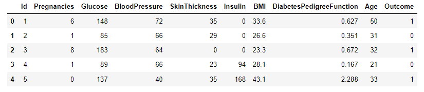
A sample dataset for diabetes classification [1] will be used to test the performance of kNN as a binary classifier. Data were extracted from 2768 patient records with mixed data of healthy and non-healthy patients inclusive of nine attributes:
Id: Unique identifier for each data entry.
Pregnancies: Number of times pregnant.
Glucose: Plasma glucose concentration over 2 hours in an oral glucose tolerance test.
BloodPressure: Diastolic blood pressure (mm Hg).
SkinThickness: Triceps skinfold thickness (mm).
Insulin: 2-Hour serum insulin (mu U/ml).
BMI: Body mass index (weight in kg / height in m^2).
DiabetesPedigreeFunction: Diabetes pedigree function, a genetic score of diabetes.
Age: Age in years.
Outcome: Binary classification indicating the presence (1) or absence (0) of diabetes.
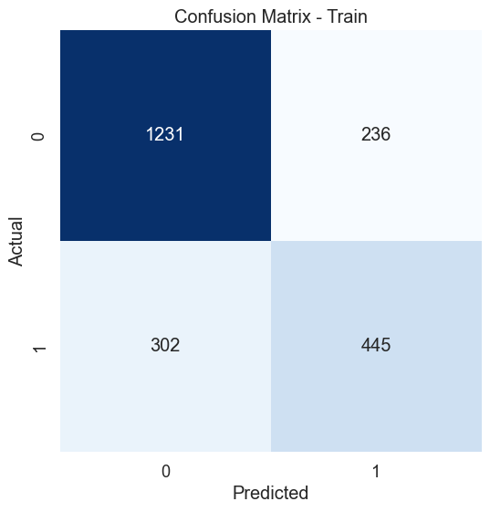
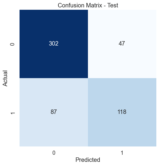
The dataset of records is split into training and test (80/20) to test the predictive performance of the Naive Bayes classifier in distinguishing between the presence or absence of diabetes. The model will thus be trained on the training set alone but benchmarked on the training and test set. The test performance is the most important as it indicates the model’s predictive power on unseen data.
import pandas as pd
import warnings
warnings.filterwarnings('ignore') #ignore warnings
df = pd.read_csv('https://raw.githubusercontent.com/mlinsights/freemium/main/datasets/classification/diabetes/Healthcare-Diabetes.csv')
X = df.iloc[:,1:9]
y = df[['Outcome']]
from sklearn.model_selection import train_test_split
X_train, X_test, y_train, y_test = train_test_split(X,y,test_size=0.2,random_state=1234)#fix the random seed (to reproduce the results)
from sklearn.naive_bayes import GaussianNB
clf = GaussianNB()
clf.fit(X_train,y_train)#train the classifier
#get model prediction on train set and test set
y_pred_train = clf.predict(X_train)
y_pred_test = clf.predict(X_test)
from sklearn.metrics import confusion_matrix
from sklearn.metrics import classification_report
import matplotlib.pyplot as plt
import seaborn as sns
import numpy as np
# Create confusion matrix for the training set
cm_train = confusion_matrix(y_train, y_pred_train)
# Create heatmap - Test set
plt.figure(figsize=(8, 6))
sns.set(font_scale=1.2)
sns.heatmap(cm_train, annot=True, fmt="d", cmap="Blues", cbar=False, square=True)
plt.xlabel('Predicted')
plt.ylabel('Actual')
plt.title('Confusion Matrix - Train')
plt.show()
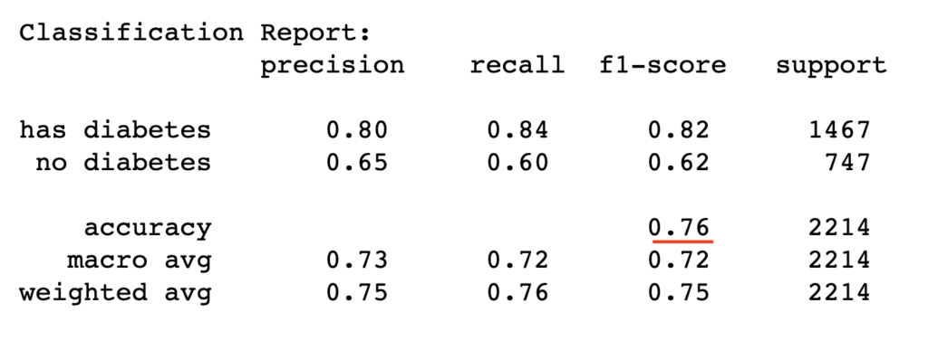
train_report = classification_report(y_train, y_pred_train, target_names=['has diabetes','no diabetes'])
print("Classification Report:\n", train_report)
# Create confusion matrix test set
cm_test = confusion_matrix(y_test, y_pred_test)
# Create heatmap - Test set
plt.figure(figsize=(8, 6))
sns.set(font_scale=1.2)
sns.heatmap(cm_test, annot=True, fmt="d", cmap="Blues", cbar=False, square=True)
plt.xlabel('Predicted')
plt.ylabel('Actual')
plt.title('Confusion Matrix - Test')
plt.show()
#tn, fp, fn, tp = cm_test
class_acc = (cm_test[0][0]+cm_test[1][1])/(cm_test[0][0]+cm_test[0][1]+cm_test[1][0]+cm_test[1][1])
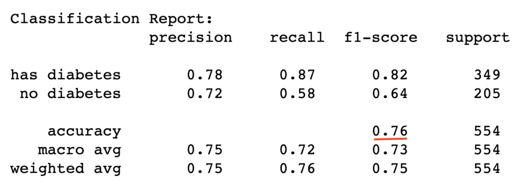
test_report = classification_report(y_test, y_pred_test, target_names=['has diabetes','no diabetes'])
print("Classification Report:\n", test_report)
Conclusion
The Naive Bayes classifier is a decent classification algorithm that relaxes the naive bayes theorem based on the assumption conditional independence of features given the class variable to devise a computable classification score. The performance of the algorithm can be improved using kernel-based density estimation to build from data the conditional probabilities of the method and yield more accurate results.