How do we determine whether a regression algorithm is performing well or not? How do we compare them against each other? Surely, this question prompts the need for some form of metrics to evaluate performance. In this tutorial, we examine the issue both philosophically and practically. Let’s dive in!
The essence of building a ML model - Training/Test Split
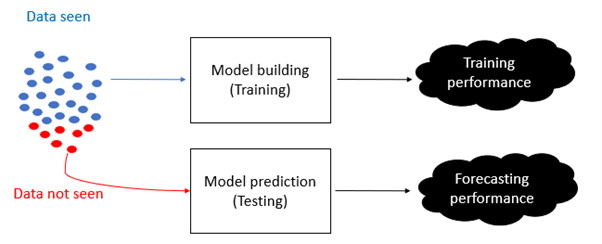
Before we dive into formulating regression metrics, we need to answer this fundamental question: Why do we build machine learning models? Well, the answer to that question is pretty straightforward but runs deep. We do build models to learn patterns, however, we are interested in accurately learning patterns on data we have not seen, rather than on data we have seen. A machine learning model will only be useful if after learning a pattern in some datasets, it can generalise and infer patterns in new data.
This justifies why while assessing the performance of machine learning models, the datasets is split into two distinct part:
Training set
Test set
The training set is used to train the machine learning model while the test set is used to assess how well the model can generalise, the most important expected outcome.
Hyperparameter tuning and the Validation Set
Besides the model parameters that are learned during data training, machine models often possess configuration parameters that are preset prior to training the model on the data. These parameters are called hyperparameters, and selecting the best parameter configuration can boost the model’s performance. This is achieved via hyperparameter tuning, a process during which several model parameters are tried on the model training set, and the model’s performance is assessed against a hold-out portion of the training set called the validation set. The validation set can also be used in some models for regularisation, ensuring that the model does not overfit, thus losing predictive accuracy.
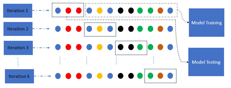
k-fold Crossvalidation - a step futher in performance testing
Keeping a hold-out data portion (i.e., validation set) from the training set is appropriate in assessing the model’s performance and generalization ability. However, a pertinent question should be asked: Which portion of the data should be used for training or validation? To fairly assess the performance of a model that may potentially display some bias in selecting one specific portion of the dataset, the k-fold cross-validation process is used. K-fold cross-validation consists of testing the model’s performance k times, whereby in each iteration, different portions of the dataset are used for training and testing.
Regression Metrics
Regression models are typically assessed using two main metrics: The coefficient of determination R^2 and the mean square error or root mean square.
The R^2 coefficient tests the goodness of fit of the model. A model with a perfect fit on the data achieves a goodness of 1, while poor models have a goodness near zero or sometimes negative.
The mean square error (MSE) assesses the average squared error between the model observation (y_i) and the model prediction. A practically relatable assessment of the model is the root mean square error (RMSE), which assesses the model error deviation against the observation. It is a measure of the model’s average prediction deviance in the same unit as the data observation.
Python Implementation - Training/Test Split
Python Implementation - k-fold cross-validation
Classification Metrics
Classification models are tested using more intricate performance indexes. Typically a classification model performance is tested using the model classification accuracy, which is the percentage of correct prediction over every data record.
\[\text{Classification Accuracy} = \frac{\text{Number of Correct Predictions}}{\text{Total Number of Records}}\]
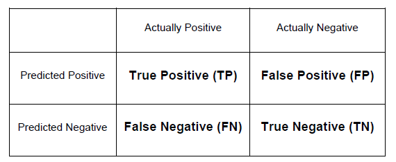
The Confusion Matrix
However, to assess the model performance more intricately, additional scores are evaluated using the confusion matrix. The confusion matrix is a table of model performance counts, including True Positive (the number of positive target observations that have been correctly classified), True Negative (the number of negative target observations that have been correctly classified as such), False Positive (the number of negative target observations that are incorrectly classified as positive predictions), and False Negative (the number of positive target observations that are incorrectly classified as negative predictions).
Computing these indexes leads to a more nuanced and intricate landscape of the performance of a classification to obtain the following scores:
Recall, also known as sensitivity or true positive rate, measures This tells the ability of a model to classify the instances of a particular class correctly.
Precision measures the accuracy of predictions made by the model. Precision indicates how confident we can be that it is actually positive. It is calculated as the ratio of true positive predictions to the total number of positive predictions made by the model. Precision answers the question: “Of all the instances predicted as positive, how many were actually positive?” It can also be applied to negative outcomes.
The F1 score is the harmonic mean of precision and recall. It provides a single metric that balances both precision and recall. The F1 score reaches its best value at 1 (perfect precision and recall) and worst at 0. The F1 score considers both false positives and false negatives, making it a suitable metric when there is an imbalance between the classes or when both precision and recall are equally important. It penalizes models with imbalanced precision and recall values.
In summary, A good model must classify all classes equally well (recall) and misclassify as little as possible (precision).
Python Implementation - Training/Test Split
#-- Load the Dataset
import pandas as pd
import warnings
warnings.filterwarnings('ignore') #ignore warnings
df = pd.read_csv('https://raw.githubusercontent.com/mlinsights/freemium/main/datasets/classification/diabetes/Healthcare-Diabetes.csv')
df.head()


#-- Summarise the Dataset
df.info()

#-- Extract Features and the target variable
X = df.iloc[:,1:9]
y = df[['Outcome']]

#-- Split the Dataset in Training and Test Set
from sklearn.model_selection import train_test_split
X_train, X_test, y_train, y_test = train_test_split(X,y,test_size=0.2,random_state=1234)#fix the random seed (to reproduce the results)
#-- Training the model
from sklearn.tree import DecisionTreeClassifier
import matplotlib.pyplot as plt
from sklearn import tree

dt_classifier = DecisionTreeClassifier(criterion="gini",max_depth=2,min_samples_leaf=1)#Setting the decision tree - settings
dt_classifier.fit(X_train,y_train)#train the classifier
# -- Benchmark the model performance
from sklearn.metrics import confusion_matrix
from sklearn.metrics import classification_report
import seaborn as sns
import numpy as np

y_pred_test = dt_classifier.predict(X_test)
# Create confusion matrix test set
cm_test = confusion_matrix(y_test, y_pred_test)
# Create heatmap - Test set
plt.figure(figsize=(8, 6))
sns.set(font_scale=1.2)
sns.heatmap(cm_test, annot=True, fmt="d", cmap="Blues", cbar=False, square=True)
plt.xlabel('Predicted')
plt.ylabel('Actual')
plt.title('Confusion Matrix - Test')
plt.show()

#tn, fp, fn, tp = cm_test
class_acc = (cm_test[0][0]+cm_test[1][1])/(cm_test[0][0]+cm_test[0][1]+cm_test[1][0]+cm_test[1][1])
test_report = classification_report(y_test, y_pred_test, target_names=['has diabetes','no diabetes'])
print("Classification Report:\n", test_report)
Python Implementation - k-fold cross-validation
Conclusion
Training a supervised learning model accurately requires a robust process that involves: splitting the datasets into training and test sets. The training set may be further split into an actual data training set and a hold-out set to identify the model’s best configuration. k-fold cross-validation may be used instead of a hold-out set (i.e. validation set) for a more unbiased assessment of the model’s predictive accuracy. Upon selection of the model’s best configuration, it may be retrained using the full training set. The constructed model may finally be tested on the test set using regression or classification metrics based on the problem at hand. This is a standard practice for effective model training.