Artificial Neural Networks (ANNs) are learning architectures that loosely mimic biological neural networks whereby many neurons, the basic unit of information processing are interconnected and acquire knowledge or skill by a process called “synaptic plasticity” which is the ability of neuronal junctions to modify their electrochemical compositions to adapt to experiences and consolidate knowledge.
Biological Neuron
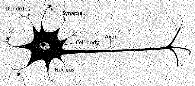
A biological neuron is made of four important parts: the nucleus which is the central repository of neuronal electrochemistry, the dendrites, neuronal input membranes, the axon, the neuron output membrane that ignites a signal when the accumulated nucleus voltage reaches a certain threshold and synapses which are inhibition and excitation joints in between neuron-to-neuron connections (i.e. dendritic to dendritic, axon to dendritic synapses).
A sketch of a biological neuron (Jain et al, 1996)
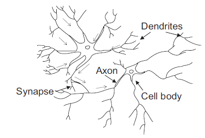
Simple neural net (Park et Lek, 2016)
Interconnected neurons will thus form biological neural networks whose learning process is based on the guided adaptability of synaptic junctions which are responsible for skill or knowledge acquisition. Thus, synaptic plasticity. Artificial neural networks will thus mimic that process.
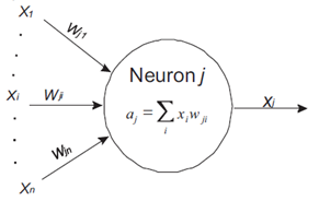
Artificial Neuron
An Artificial neuron is a simplified biological neuron that focuses on the learning paradigm. The dendrites are replaced by input variables (x_i), the synapses are replaced by numerical weights, that adaptively accumulate input signals as a weighted sum.
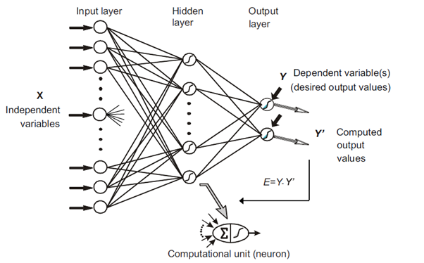
Also called multilayer perceptrons (MLP), feed-forward neural networks are very popular artificial neural networks (ANN) with only forward connections that are used for a wide variety of problems, they are universal approximators that can be used for both regression and classification and learn very complex nonlinear relationships.
Multilayer Perceptrons (Park et Lek, 2016)
Training ANNs - The Backpropagation method
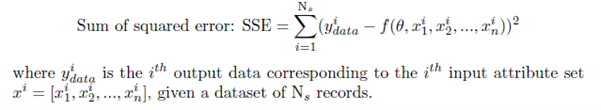
Similarly, to common parametric supervised learning models, training MLPs refers to minimising the discrepancy between the prediction and the real data output across all data records.
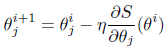
The backpropagation method, an adapted gradient descent algorithm that uses the chain rule is used to estimate the huge number of parameters int the feedforward neural network.
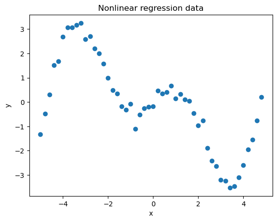
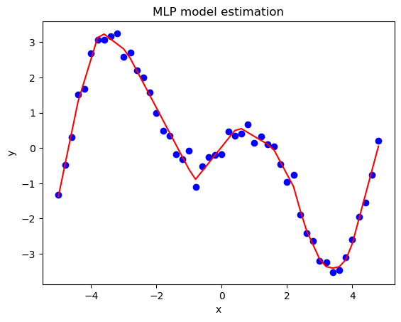
To illustrate the pattern discovery prowess of neural networks, an MLP will be trained to estimate the nonlinear relationship in regression data. A typical linear regression will not accurately estimate the existing relationship in the current dataset. However, using an MLP as a universal regression approximator, the inherent pattern can be deciphered.
import pandas as pd
import matplotlib.pyplot as plt
import warnings
warnings.filterwarnings('ignore') #ignore warnings
from sklearn.neural_network import MLPRegressor
from sklearn.preprocessing import StandardScaler


df = pd.read_csv('https://raw.githubusercontent.com/mlinsights/freemium/main/datasets/regression-analysis/1d_nonlinear_regression_data.csv')

x = df[['x']]
y = df[['y']]

#standardise the input feature for accurate modelling
scaler = StandardScaler()
scaler.fit(x)
xs = scaler.transform(x) #generate standardised input feature

#MLP with 1 hidden layer of 20 neurons
clf = MLPRegressor(hidden_layer_sizes=(20),max_iter=1000,
                  early_stopping=False,activation='relu',solver='lbfgs')

#traing MLP model
clf.fit(xs,y)

#predict the observation data
y_pred = clf.predict(xs)

plt.figure()
plt.scatter(x,y,color="blue")
plt.plot(x,y_pred,color="red")
plt.xlabel('x')
plt.ylabel('y')
plt.title('MLP model estimation')
plt.show()
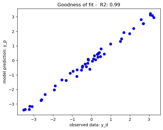
Goodness of fit - Coefficient of determination R2 score
Similarly to any regression algorithm, the goodness of fit between the observation data and model prediction including the coefficient of determination (R2 score) will evaluate how well the data fitting process has been. More information of the estimation of this coefficient can be found under linear regression.
from sklearn.metrics import r2_score

r2_score_m = r2_score(y_pred,y)

plt.figure()
plt.scatter(y, y_pred, color="b")
plt.xlabel('observed data: y_d')
plt.ylabel('model prediction: y_p')
plt.title('Goodness of fit -  R2: %.2f'%r2_score_m)
plt.show()
Conclusion
This tutorial has introduced the topic of artificial neural networks with a particular emphasis on the popular architecture of feedforward neural networks. Neural networks are both able to detect very complex relationships and are at the same time prompt to overfitting especially for problems that require generalisation on test datasets. Proper training, regularisation and validation approaches are needed to prevent overfitting. Other neural network architectures exist such as convolutional neural networks (CNN), and recurrent neural networks (RNN) are more suited for specific types of problems such as image recognition time series analysis, or audio patterns and more.
Author: Yves Matanga, PhD
References
[1] Jain, A.K., Mao, J. and Mohiuddin, K.M., 1996. Artificial neural networks: A tutorial. Computer, 29(3), pp.31-44. [2] Park, Y.S. and Lek, S., 2016. Artificial neural networks: Multilayer perceptron for ecological modelling. In Developments in environmental modelling (Vol. 28, pp. 123-140). Elsevier.
Be the first to receive notification, when new content is available!